Forecasting Tesla (TSLA) Stock Prices with Prophet and Python

Disclaimer This prediction model is designed for educational and learning purposes only. We are not responsible for any losses incurred when using it for actual investment purposes. Please consult with a professional before making any investment decisions and exercise your own discretion.

Important Limitations of Prophet for Stock Price Prediction

Prophet models cannot account for critical market factors:

• Corporate Earnings Reports: Quarterly results, guidance changes, and surprise announcements
• Economic Indicators: Interest rates, inflation data, GDP growth, unemployment figures
• Geopolitical Events: Trade wars, regulations, political instability, international conflicts
• Market Sentiment: Investor psychology, fear/greed cycles, social media trends
• Industry Trends: Technological disruptions, competitive dynamics, sector rotations

Key Takeaway

This model is designed for educational and demonstration purposes only.
DO NOT use these predictions for actual investment decisions.
Stock prices are influenced by countless external variables that time-series models cannot capture.

For production use, consider:

• Incorporating fundamental analysis
• Adding technical indicators
• Using ensemble models (LSTM, Transformer, etc.)
• Integrating news sentiment analysis
• Applying risk management strategies

Introduction

• TL;DR: This article provides a complete walkthrough of forecasting Tesla (TSLA) stock prices using Python. We use the yfinance library to fetch historical data and Meta’s Prophet library to build a time-series prediction model. The process covers data acquisition, preprocessing into Prophet’s required ds and y format, model fitting, and visualizing the forecast, including trend and seasonality components. It’s a practical guide for practitioners starting with financial data analysis.

Step 1: Setting Up the Environment

First, we need to install the necessary Python libraries for our analysis. yfinance is for fetching stock data, prophet is for forecasting, pandas for data manipulation, and matplotlib for plotting.

1

!pip install yfinance prophet pandas matplotlib -q

Once installed, import them into your Python script or notebook.

1
2
3
4

import pandas as pd
import yfinance as yf
from prophet import Prophet
import matplotlib.pyplot as plt

Why it matters: A properly configured environment is the foundation for reproducible and error-free analysis. Each library plays a specific role, and ensuring they are all installed correctly prevents issues later in the process.

Step 2: Fetching Tesla Stock Data with yfinance

We use yfinance to download historical stock data. The ticker symbol for Tesla is TSLA. We’ll download the data for the last five years.

1
2
3
4
5
6
7
8

# Define the ticker and date range
ticker = 'TSLA'
start_date = '2020-01-01'
end_date = '2025-10-10'

# Download the data
data = yf.download(ticker, start=start_date, end=end_date)
display(data.head())

Why it matters: The quality of a predictive model heavily depends on the quality of the input data. yfinance provides a simple and standardized way to access reliable historical financial data with just a few lines of code.

Step 3: Preprocessing Data for Prophet

Prophet requires the input DataFrame to have a specific structure: a ds column for the datestamp and a y column for the value we want to forecast (the closing price).

Python

 1
 2
 3
 4
 5
 6
 7
 8
 9
10
11
12
13
14
15
16
17
18
19
20
21

# Convert date index to column
df = data.reset_index()

# Select required columns and rename them
df = df[['Date', 'Close']].rename(columns={'Date': 'ds', 'Close': 'y'})

# Handle MultiIndex columns issue (due to yfinance data structure)
if isinstance(df.columns, pd.MultiIndex):
    df.columns = df.columns.get_level_values(0)

# Convert ds column to datetime format
df['ds'] = pd.to_datetime(df['ds'])

# Convert y column to numeric and flatten
df['y'] = df['y'].values.flatten()

# Remove NaN values
df = df.dropna()

# Check the data
print(df.sort_index(ascending=False).head())

Why it matters: Data preprocessing is a critical step in machine learning. Adhering to the model’s expected input format is essential for the training process to run without errors.

Step 4: Training the Model and Making Predictions

With the data prepared, we can create and train our Prophet model. Since Tesla is a U.S. stock, we will include holidays for the United States.

 1
 2
 3
 4
 5
 6
 7
 8
 9
10
11
12
13

# Enhanced Prophet model (more sensitive to trend changes)
model = Prophet(
    daily_seasonality=True,
    changepoint_prior_scale=0.5,  # Set higher than default 0.05
    seasonality_prior_scale=10,
    changepoint_range=1.0  # Detect changepoints across 100% of data
)

# model.add_country_holidays(country_name='KR')  # Add Korean holidays
model.add_country_holidays(country_name='US')  # Add US holidays

# Train the model
model.fit(df)

Next, we create a “future” DataFrame to hold the dates for which we want predictions. Let’s forecast for the next 365 days.

 1
 2
 3
 4
 5
 6
 7
 8
 9
10
11
12
13
14
15
16
17
18
19
20
21
22
23
24
25
26

# Create dataframe for 365-day future prediction
future = model.make_future_dataframe(periods=365)

# Execute prediction
forecast = model.predict(future)

# Check the last date of original data
last_date = df['ds'].max()
print(f"Last date of original data: {last_date.strftime('%Y-%m-%d')}")
print(f"Last actual closing price: ${df[df['ds'] == last_date]['y'].values[0]:,.2f}\n")

# Filter only future predictions
future_forecast = forecast[forecast['ds'] > last_date].copy()

# Compare with recent actual data to verify prediction accuracy
recent_actual = df.tail(5)[['ds', 'y']].rename(columns={'y': 'actual'})
recent_forecast = forecast[forecast['ds'].isin(recent_actual['ds'])][['ds', 'yhat']]
comparison = recent_actual.merge(recent_forecast, on='ds')
comparison['error'] = ((comparison['yhat'] - comparison['actual']) / comparison['actual'] * 100)

print("=== Recent Prediction Accuracy ===")
display(comparison)

print(f"\n=== Future Predictions (Next 10 Days) ===")
print(f"Prediction start date: {future_forecast['ds'].min().strftime('%Y-%m-%d')}")
display(future_forecast[['ds', 'yhat', 'yhat_lower', 'yhat_upper']].head(10))

Why it matters: This is the core of the forecasting process. Prophet simplifies the complex tasks of model fitting and prediction generation, allowing developers to quickly build and evaluate forecasting models.

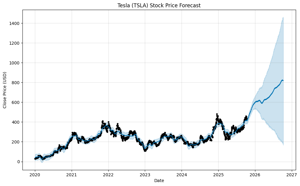
Step 5: Visualizing the Forecast

Visualization helps in understanding the model’s performance and the nature of the forecast. Prophet has built-in plotting functions to make this easy.

Python

1
2
3
4
5
6

# Plot the forecast
fig1 = model.plot(forecast)
plt.title('Tesla (TSLA) Stock Price Forecast')
plt.xlabel('Date')
plt.ylabel('Close Price (USD)')
plt.show()

To better understand the components of our forecast, we can use plot_components.

1
2
3

# Plot the forecast components
fig2 = model.plot_components(forecast)
plt.show()

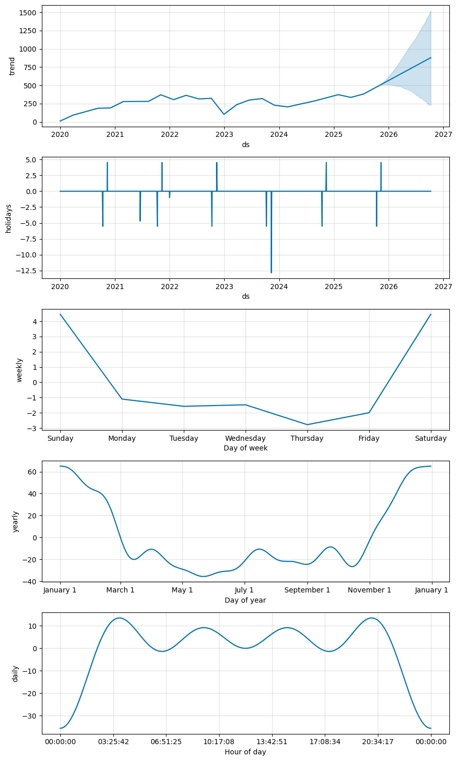
Why it matters: Visualization translates raw numbers into an intuitive format, making it easier to assess the forecast’s quality and understand the underlying trends and seasonal patterns that the model has identified.

Conclusion

This guide demonstrated how to build a time-series forecasting model for Tesla’s stock price using Python, yfinance, and Prophet. While this example provides a solid foundation, it’s crucial to remember that stock market prediction is incredibly complex and influenced by numerous factors not included in this model.

• Key Takeaways:
  • yfinance provides an easy interface to download historical stock data for tickers like TSLA.
  • Prophet requires data in a specific ds and y format.
  • The entire process involves data fetching, preprocessing, model fitting, and visualization.
  • This model is for educational purposes and should not be used as financial advice.

Summary

• Fetched Tesla (TSLA) stock data using the yfinance Python library.
• Preprocessed the data into the ds (date) and y (close price) format required by Prophet.
• Built and trained a Prophet model, including seasonality and U.S. holiday effects, to forecast prices for the next 365 days.
• Visualized the final forecast and its underlying components (trend, weekly/yearly seasonality).